Simplified understanding of Retrieval Augmented Generation (RAG)

Introduction

Image Generated with the prompt info extraction from document

One of the interesting applications of Generative AI is searching for information within your own documents which is termed as Retrieval Augemented Generation or RAG in short. There are many different combinations and software to setup a RAG on a local system. the ability to perform RAG entirely on a local system looks to be slightly more challenging. In this article, we would like to share on some of the more simple and straightforward ways RAG can be implemented on a local machine without the need to call an API over the internet.

Most straightforward - Install directly from NVIDIA

The most straightforward way to experiment chatting with your documents is with the NVIDIA tool ChatRTX demo app which can be downloaded from the NVIDIA website and installed directly. More details about the tool can be found at https://www.nvidia.com/en-us/ai-on-rtx/chat-with-rtx-generative-ai/

High Level illustration of RAG

Simplified Overview of a RAG system end to end

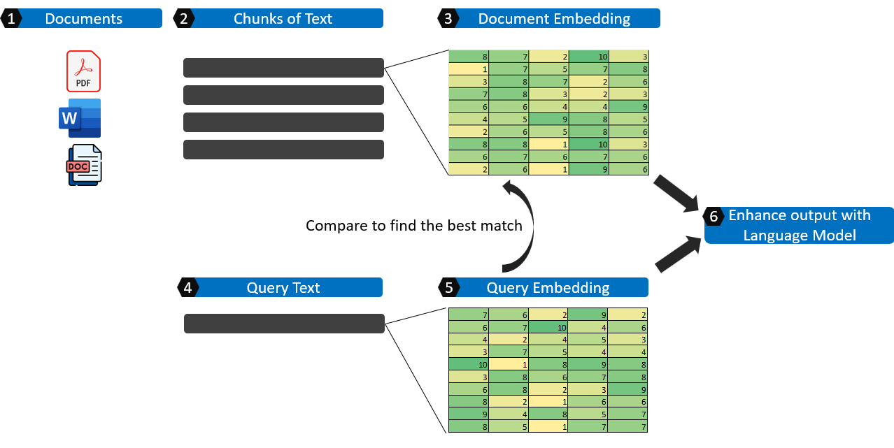
There are many useful blogs and resources explaning about Retrieval Augmented Generation (RAG) and this is my attempt to explain it in simple terms with the basic components.

1. In the first step, relevant text is extracted and consolidated from the source documents.
2. These documents are broken up into chunks, logical smaller pieces of information.
3. Each of the text in the chunk is transformed into an embedding which is essentially representing the text in numbers and is usually in a matrix format.
4. We get the query text.
5. The query text is also transformed into an embedding and is compared against the collection of document embeddings to find the most relevant chunks of text.
6. The query, together with the relevant chunks of text are fed into a Large Language Model as part of the context to output a coherent response.

Similarity matching of sentences

For a retrieval augemented generation, there will be a base collection of information sources which can come from documents, online faqs, text information in a database etc. The documet will be broken up into smaller chunks and an embedding will be generated for each chunk. The query will then be compared against each chunk of information and find the top number of most similar results.

Basic similarity using Jacquard Similarity

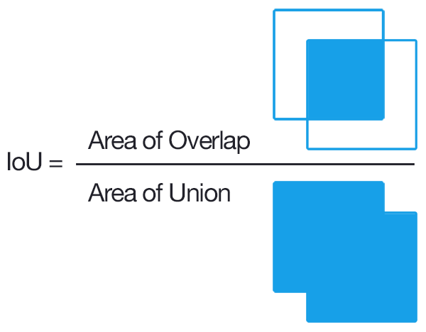
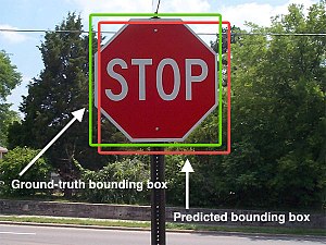
Taking inspiration for an article on the basics of RAG https://learnbybuilding.ai/tutorials/rag-from-scratch, one of the common methods of measuring similarity is using Jacquard similiarity which is employed for the evaluation of object detection algorithms. The image below shows a graphical overview of how the jacquard similarity coefficient is calculated.

Jacquard similarity coefficient calculation

Jacquard similarity used in object detection

First we have a collection of sentences to from a corpus. In our simple example, the corpus consist of four sentences with the first three having the same meaning, being the paraphrase of each other while the last sentence has the opposite meaning to the first sentence.

corpus_of_documents = [
    "The forecast predicts heavy rain for the entire week.",
    "A week of intense rainfall is expected according to the weather report.",
    "The weather outlook indicates a week-long period of intense rainfall.",
    "The weather report anticipates dry weather throughout the week."
]

Next we define the simple functions to calculate the coefficients and find the closest sentence.

def jaccard_similarity(query, document):
    query = query.lower().split(" ")
    document = document.lower().split(" ")
    intersection = set(query).intersection(set(document))
    union = set(query).union(set(document))
    return len(intersection)/len(union)

def return_response(query, corpus):
    similarities = []
    for doc in corpus:
        similarity = jaccard_similarity(user_input, doc)
        similarities.append(similarity)
    return corpus_of_documents[similarities.index(max(similarities))]

We compare the sentences to a sample query: “The forecast predicts dry weather for the week.”. As we can see, based on the similarity using jacquard coefficent, it is not so useful for finding sentences with the same meaning since the sentence output is the opposite of the query. It is more about finding sentences with the highest proportion of words in common.

Output from Jacquard Similarity function

Similarity matching based on sentence embedding

For the concept of embedding, I found that Jeremy Howard explains it best in his free course and the link to the lesson can be found here: https://course.fast.ai/Lessons/lesson7.html. In his lecture, he explains about embedding through the recommendation systems technique, collaborative filtering, which is about creating numeric representations of users and movies based on their interactions. In a similar manner, words and their positions can be transformed into a numeric representation. More details about sentence embedding can be found in https://docs.cohere.com/docs/text-embeddings

Using embeddings, the matching of similar sentences based on their meanings become more accurate. Some of the popular models in terms of the speed of inference and model accuracy can be found at the Sentence Bert webiste https://www.sbert.net/docs/pretrained_models.html. Using the all-MiniLM-L6-v2 model which is one of the most common starting models, we are able to get a more accurate search somewhat based more on meanings rather than purely common words as shown below.

from sentence_transformers import SentenceTransformer, util
# Initialize the model
model = SentenceTransformer('all-MiniLM-L6-v2')
# Convert list of sentences into embedding
corpus_embeddings = model.encode(corpus_of_documents)
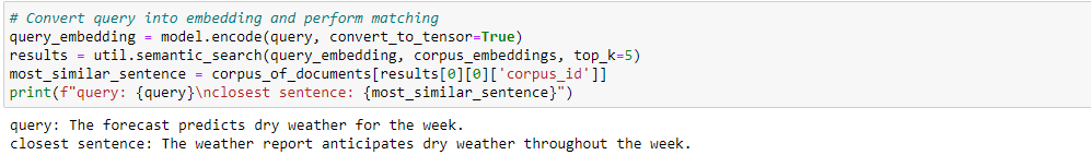
# Convert query into embedding and perform matching
query_embedding = model.encode(query, convert_to_tensor=True)
results = util.semantic_search(query_embedding, corpus_embeddings, top_k=5)
most_similar_sentence = corpus_of_documents[results[0][0]['corpus_id']]
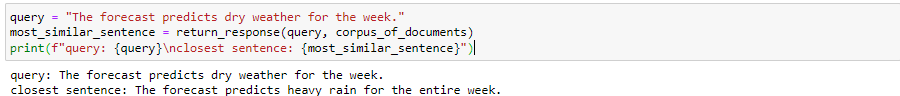
print(f"query: {query}\nclosest sentence: {most_similar_sentence}")

The output from the sentence embedding code is shown below. We can see that the closest matching sentence from the sentence embedding is not only dependant on the number of common words.

Output from sentence embedding similiarity matching

Feeding the query and context into a Language Model

Once the top closest items are generated, they can be prepared as context as input to feed into a language model. That combined with the query are fed into a language model usually in a format optimized for RAG. An example can be found below:

qa_prompt_tmpl_str = (
    "Context information is below.\n"
    "---------------------\n"
    "{context_str}\n"
    "---------------------\n"
    "Given the context information and not prior knowledge, "
    "answer the query.\n"
    "Query: {query_str}\n"
    "Answer: "
)

Next Steps

In this article, we examined the foundational concept of similarity matching and preparation of the context together with the query to be fed into a Large Language Model (LLM). There has been many developments in terms of making LLMs more efficient or quantizing a LLM such that it can be run on a local machine even without GPU. We target to follow up with the next article on the simplest way to implement a RAG solution locally ideally using a CPU for inference.